A Full-Featured Open-Source Framework for Image Processing

Road Systems, Maybe, or Cells

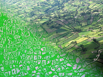Commonalities among seemingly unrelated things always intrigue. The lay of the land around Ipiales, Colombia at three hundred meters' height has similarities with photomicrographs of plant stem tissue. They hint at universal rules governing how areas and volumes apportion themselves. The wealth of property owners, topographical features and human politics conspire in particular ways to shape pastures and roads. Similar logistics affect cell growth. Cell size and shape are limited by the availability of nutrients, signalling from other cells and their own DNA "software." This recipe apes such logistics. It generates a mask that may support a larger project. The mask divides a surface into irregular cobblestones — perhaps — or cells, or pastures nestled between roads.

Consider this custom command, which makes such a mask:

---

-noise_poissondisk[canvas] 20,30,2 A sparse scattering of white pixels — spikes — plotted through the courtesy of the noise_poissondisk command. This command strives for a distribution that exhibits minimal low frequency components; noise spreads evenly across every region. Compare with the similar (and faster) built-in command, noise: gmic run '-input 256,256,1,1 -noise. 0.20,2 abs.' Overall, its noise distribution may be similar, but the built-in admits both clumped and overly sparse regions; within such variations a spectrally attuned eye senses low frequency components. Why would such variations matter? Noise is the core ingredient in many procedural texture recipes — which is what we are conjuring here — and how one starts out very much affects how one finishes. If the texture is to resemble fish scales, noise_poissondisk is likely the better choice. Soiled fabric? Probably then -noise, since dirt favors clumping. Target distance: The first argument to -noise_poissondisk — 20 — sets a target distance, this to be maintained in separating spikes. Larger values lead to more sparse distributions. Trials: The second argument — 30 — sets the number of trials undertaken in the search for uniform separation. Should this value be very small, say 1 or 2, then the noise distribution will not be especially uniform. Typically, "holes" form in the distribution. Larger trial values lead to better results, but improvements level off; very large trial values, like 100, obtain nearly undistinguishable results from 30, this for images with dimensions around 1000 pixels. The optimal trial number tends to increase with image size. Measure: The third argument may intrigue. It chooses a distance function from the family of Lp measures. Pray, what is that? We seek recourse to distance functions ( measures ) to tell us how far apart two given points are. The measure need not be the usual Euclidean distance function, , familiar though that may be. We can hold the distance from Turtle Bay to Times Square in Manhattan to be "as the crow flies," but we're not crows and the airspace above Manhattan is restricted. So, we have to hoof it — on the surface — and the rectangular street grid limits our traversals to east-west or north-south directions. This, in fact, is the Manhattan measure. We just sum the absolute values of our north-south, east-west perambulations and leave it at that: no squaring of terms, no square roots of aggregates. In cityscapes, this approach happens to provide a more practical measure of "distance traveled" than a Euclidean "as the crow flies" measure, one that serves the reality of grid-locked Manhattan. And so it goes: we choose whatever measure that best fits the nature of the space we're in. For noise_poissondisk, this choice affects how the command arrives at "uniformly spread noise spikes", which entails comparing many, many distance measures. 2, the default argument, selects the L2 norm. This corresponds to the Euclidean distance function. 1 selects the L1 norm — the Manhattan measure. And, generally, argument p selects:

the Lp norm on an n dimensional space. For p>2, noise_poissondisk operates within non-Euclidean realms, but the intrinsic operation of the command remains unaltered. Poetically, with these various Lp measures, we choose how the "fabric of space" transmutes, giving rise to subtle fluctuations in the scatter of points.

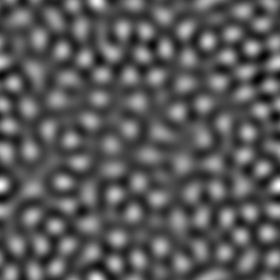	Minimum and Maximum Frequency: The -bandpass[canvas] 0.001,0.009 command transforms an image to and from the complex frequency domain. In the midsts of that transit, it zeros out all frequency domain coefficients but those occupying a ring defined by inner and outer radii, here 0.001 and 0.009. These set lower and upper extents of a passband, the interstice between the radii. These arguments are very nearly the same and small, delineating a spectral realm that selects just long wavelength spatial signals. On the back transition, only the selected low frequency waveforms appear, their interference pattern bringing into being the image. That is all that remains of the spikes generated by noise_poissondisk, the road system — or cell pattern — is latent within. Being periodic along the x and y axes, the image readily makes seamless tiles, a desirable texture property. By fiat, the most luminant regions of this interference pattern become cell bodies — or hills among roads (it could also be the other way around). The follow-on commands bring forth this latent topology.
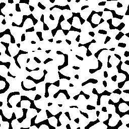	Threshold the Extremes: By thresholding, we've done some setup for the follow-on -thinning command. The cut-off at 25% of the range abs(iM–im) was chosen because it produces an image where very nearly all white pixels are contiguous, while the black regions tend to disjointness. With the ideal, one can travel from any white pixel to any other without crossing a black region. Being near a cusp, 25% is likely near — but not at — this ideal.
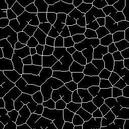	Bring Forth The Roads: -thinning morphologically advances black — logical 0 regions — into white (logical 1) until the latter become one-pixel-wide lanes; black regions can advance no further. It is this command that, roughly speaking, sets up a kind of competition which allies these images to cell tissues or plots of land; the separating lanes prototype cell walls or roads — take your pick. This is a substantially time-consuming command, given per-pixel testing along advancing fronts, but — alas! — lies at the very heart of this road/cell texture.  competition is preordained in favor of the larger, wealthier black pockets. Eventually, colliding upon the ridges, all frontal movement is arrested. This leaves a set of parcels, each encompassing a black region. The smaller parcels range very little to begin with and cannot expand like the larger ones.
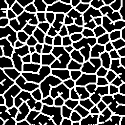	Dilatory Passages: -dilate_circ[canvas] 4 and the following-on blur and threshold commands serve artistic interests. Having choked roadways (or cell walls) within a pixel of their lives, we dilate the passageways (or walls) with another morphological transform, this emulating a circle with a four pixel diameter sweeping down the passage ways (walls).
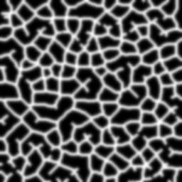	Rounding the Shoulders: Nature tends to abhor sharp transitions. Here, -blur[canvas] 2 sets up a second use of threshold. Together, this command and its follow-on reduce unlikely sharp corners. With thresholding, the blurred corners emerge rounded, emulating real-world corner-cutting as people tread on grass; corners always wear more than straghtaways.
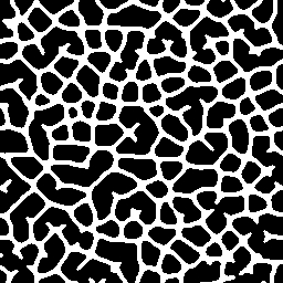	Making the Mask: Thresholding completes the mask, and we are — almost! — done. Practicalities intrude. First, the mask is made up of one and zero pels, logically satisfying, but this last image on the stack does not play well with paint programs. As noted in Images as Datasets the output of G'MIC commands may not be apt for post-processing in paint programs. -normalize[canvas] 0,255 serves no other purpose than to relocate the mask into the range of 0,255, suitable for unsigned eight byte file formats and the subsequent use in paint programs.

Finger Exercises

As written, this texture generator is a bit inflexible. Wider roads? Bigger islands? roadsorcells billets none of that. That said, custom commands take arguments, the basis for finger exercises.

New to G'MIC? The technique is simple. In pipelines, arguments follow commands; these are set off by one or more spaces and form comma-separated argument lists. Collateral $-expressions inhabit the custom commands themselves; these are placeholders which G'MIC substitutes with argument values. These placeholders consist of dollar signs $ followed by numerals, each matching a position in the argument list. $0 placeholds for the name of the custom command: roadsorcells; $1 placeholds for first argument and so on. There are other $-expressions; these provide various argument list properties. Command Arguments plunges into details.

Here, we have modified roadsorcells.gmic to accept two optional arguments, setting the lower and upper extents of the passband. If we do not provide arguments — or provide only one or the other argument — the custom command applies pre-defined defaults. The custom command also scales these arguments so that the command's user can operate with larger values than itty-bitty fractions — with lots of leading zeros that are so convenient to miscount.

With roadsorcells so modified, we can illustrate the effects of increasing passbands:

So goes the parameterization of passband arguments. A mathematical expression, {2*$>} computes the second one such that the upper frequency limit of the passband advances by twice the loopcount: $>. This is a common use of mathematical expressions: setting up ranges of argument values, an investigation of behavior that goes hand-in-hand with finger exercises.

Counterintuitively, the more tightly-spaced bandpasses give rise to larger cells, hills or islands (take your pick): an inverse relationship. Such is the manifestation of spectral domain operations where tiny distances from the origin imply spatially long-wavelengths; roadsorcells primarily processes the interference patterns of such.

We may also parameterize other command aspects but now trust in an established grasp of the technique. he key takeaway bit is how unexpected behavior oft-times emerges from range checking. It can be easily overlooked, but — when noticed! — may be capitalized in visually interesting ways.

Updated: February 5, 2024 18:30 UTC Commit: ceda63b2867a